

All about Advanced Filter in Excel- User interface
- V E Meganathan
- Apr 23, 2024
- 4 min read
Today we are going to discuss about advanced filter - user interface option in excel. This is not dynamic like formula but can-do complex filters with ease which we can't do using regular filter option. You will see some cases with formulas in advanced filter option.
Lot to learn, let's dive in.
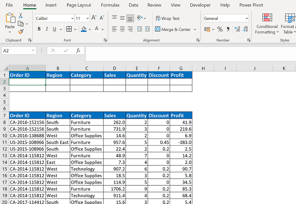
Our source data is in the range A7:G32. Criteria range is A1:G3. Instead of all column headers, we can even use one column header in criteria range based on our requirement. But the column header in criteria should match with column header in source data.
Best practice is to keep the criteria range above our data.
To apply advanced filter and to get the filtered result in same sheet,
click inside the data,
In menu bar -> Data tab -> Sort & Filter group -> Advanced filter
else use shortcut key Alt + A + Q, below dialog box will open.

We can apply filter in the same range like, basic filter or we can select Copy to another location in action area.
Once we select that option,
we can see that list range is detected automatically, we can resize the range or we can give new range based on our requirement.
We will discuss each of this with examples.
Method 1:
Use advanced filter to get unique values in region column.
We can do that in numerous methods in advanced filter, let me show you 2 methods.
Without criteria range,
Select any one cell in data and press Alt + A + Q shortcut key,

In advanced filter dialog box, select Copy to another location, and in the list range make sure, we select only the region column. No need of criteria range here.
Then in Copy to range, select any cell, in our case we selected J7 cell.
Check the box for Unique records only and click OK.

With criteria range,
Use below formula in J2 cell,
=COUNTIF($B$8:$B8,B8)=1
make sure, the cell above this formula cell is blank. Excel will consider that blank cell as header and will apply this formula in each cell in list range.
Make sure that the output of the formula is a Boolean value.

Arguments of COUNTIF function,
=COUNTIF(range,criteria)
What this formula does?
range in this formula is expandable range,
In B8 cell, range is $B$8:$B8, if we evaluate that, then the result is {"South"}.
Criteria is "South".
How many "South" is there in "South"? result is 1 and so TRUE.
In B9 cell, range is $B$8:$B9, if we evaluate that, then the result is {"South","South"}.
Criteria is "South".
How many "South" is there in that list? result is 2 and so FALSE.
In B10 cell, range is $B$8:$B10, if we evaluate that, then the result is {"South","South","West"}.
Criteria is "West".
How many "West" is there in that list? result is 1 and so TRUE.
If we pick the cell values corresponds to TRUE, we can get unique values.
Now get back to Advanced filter,
Select any one cell in data, and press shortcut key Alt + A + Q,

Select Copy to another location,
Make sure only range column is selected for list range,
Criteria range is $J$1:$J$2, Copy to range is $J$7 and click OK. What you did is a magic.
Method 2:
Use advanced filter with one criteria in region column.
We are going to extract the records for the region south.

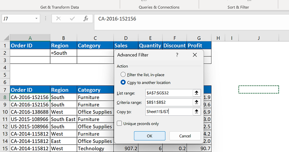
As usual select Copy to another location,
In list range select entire data,
Criteria range select B1:B3 and copy to range is J7 and click OK.

Oh, my goodness! records related to Southeast is also getting extracted.
Default option in Advanced Filter for the criteria is 'Begins With', not the exact match.
Since 'South East' begins with 'South', those records are also displayed.
If we want exact match, then simply do this in criteria range,
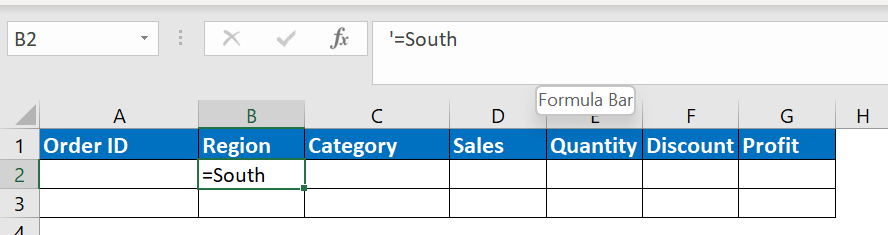
Now, we can see the records related to South region only.
Method 3:
We are going to extract the records for the sales value is less than or equal to 250.

The result is shown below,

Method 4:
We are going to extract the records for the sales value is greater than 250 and less than 1500. Two conditions in the same column, can we do it here?
No issue, add one more column header for sales as shown below.
Criteria in adjacent columns are considered as AND condition.
Criteria in adjacent rows are considered as OR condition.

Result of this filter is shown below.

Method 5:
We are going to see both AND, OR conditions now.
Our requirement is to apply filter for below criteria,

Here, the criteria are,
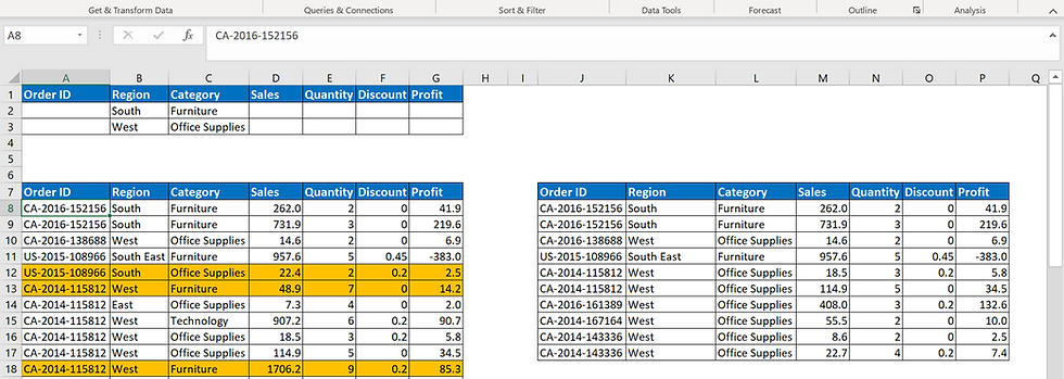
Region South AND Category Furniture OR
Region West AND Category Office Supplies.
Each record in our final output has to have south region and furniture category or
West region and category office supplies.
We cannot use this condition in our basic filter.
Let's see why.

Take a look at the highlighted record at row number 12. This does not meet our criteria. For the south region category can only be furniture. But if we apply the basic filter, this record will be included in filtered result as shown below. In that case, advanced filter and formula solution comes to rescue.
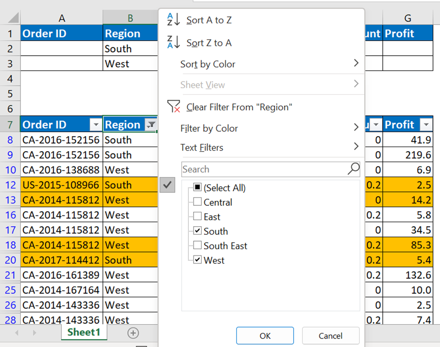

See left side picture for region filter, and right-side picture for category filter.
So, basic filter produces incorrect output as result.

Now, advanced filter in rescue,

Correct result as output.


Comments