

Dependent drop down list in Excel using OFFSET function
- V E Meganathan
- Apr 3, 2024
- 3 min read
Today we are going to discuss about creating data validation list from basic drop down to dependent drop down in excel. Lot to learn, let's dive in.
By default in excel, data validation set to allow any value in all cells. That's why we are able to enter texts, numbers, Boolean values, errors and so on.
Our requirement here, is to set the data validation in cell, only to allow the list of our desired values. Before that, let me show you the requirement and expected output.


Here, we have to prepare 2 drop downs, one is for Quarters in F3 cell and the other is for months in F6 cell, which will be dependent on Quarter selection.
Let me start with drop down for Quarter selection,
Copy the data from A3:A15 and paste in D3 cell. To get the unique items from that list, select the range from D3:D15 and press Alt + A + M to remove the duplicates.
Now, select F3 cell, in the data menu, data tools group, you can see the small drop down, click on that to see data validation option, click on that as shown below.

Data validation dialog box will open, ensure that settings tab is selected, otherwise select Settings tab at top right corner. Click the drop down in allow and select List option.

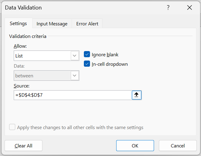
Then, click on the up arrow button for source and select the range from D4:D7 and click OK.

Now, if we select F3 cell, you can see that drop down option is enabled. We can only select any of the options in drop down in that particular cell, if we try to enter values other than in drop down, excel will not allow. This is the basic form of data validation with list range.
Then we are going to move into next stage of data validation.
Formula in F6 cell is,
=OFFSET(Sheet1!$B$3,MATCH(Sheet1!$F$3,Sheet1!$A$4:$A$15,0),,3,1)
The arguments of OFFSET function are,
=OFFSET(reference,rows,cols,[height],[width])
This function has 5 arguments and each of the argument can move in all directions, that's why this is so powerful when it comes to dynamic range. But this is a volatile function.
That means, it will recalculate whenever you press enter in any of the open excel workbook.
So, there is a bit of concern when it comes to speed. If we are aware about that, then we can use the flexibility of this function. Since we are going to use that in named range, ensure that necessary reference locking's are done.
In our case, we fed $B$3 cell as input for reference argument, rows argument helps us to move up or down from the reference range. Here, we used MATCH function to get the starting position of the dynamic range.
If we put Q1 in F3 cell, MATCH function will pick that value as lookup value and match it in the range A4:A15. Q1 is there in the first position, so, MATCH function will deliver 1,
If we put Q2 in F3 cell, MATCH function will pick that value as lookup item and match it in the range A4:A15. Q2 is there in the 4th position, so MATCH function will deliver 4 and so on.
Since our origin position is in B3 cell, we don't need to offset columns, so either we can ignore columns argument, or we can feed 0.
Then for height argument, we hardcoded the input as 3, this is because every quarter has 3 months anywhere in the world (Hardcoding is not entertained here, but for the sake of making it easier for you to understand).
For the width argument, we fed 1 since we need only one column.
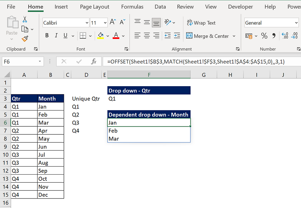
So, finally what offset does is that, if Q1 is selected, then it will start at B4 cell and pick 3 row * 1 column. If Q2 is selected, it will start at B7 and pick 3 row * 1 column. In that way, we can get the desired months based on Quarter selection.

Now, copy whole formula and keep the F6
cell as active cell, then click on the 'Formulas' tab in the menu bar and select 'Name Manager'. Click New in dialog box.
'New name' dialog box will open, in that set the name as 'Dep_Drop' and in the refers to section paste the formula and click OK. In Name Manager dialog box click Close.

Delete the formula in F6 cell, then do the data validation process as instructed above till the source selection step. Instead of range selection, click inside the source selection box and press F3 to open 'Paste Name' dialog box. In that, select 'Dep_Drop' and click OK.

In the Data validation dialog box, click OK.
Now, you can see that data validation in F6 cell is dynamic and dependent on F3 cell selection.
Comments