

Different Methods in Excel to find the last non-blank cell with text or number or any value
- V E Meganathan
- Sep 10, 2024
- 2 min read
Today we are going to discuss about different methods in Excel to find the last non-blank cell with text or number or any value in a given range. Lot to learn, let's dive in.
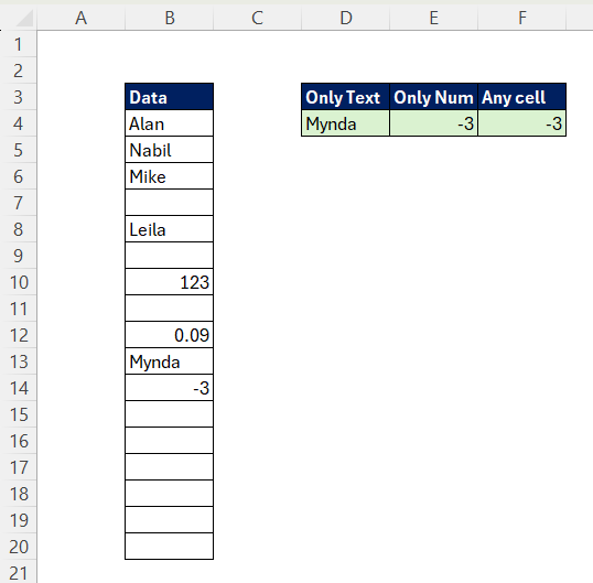
Input data resides in the range B4:B20, which contains texts, numbers and blanks.
Let me start with methods to find text values.
Method-1:
Formula in D4 cell is,
=LOOKUP(REPT("z",5),B4:B20)
Syntax of LOOKUP function,
=LOOKUP(lookup_value,lookup_vector,[result_vector])
=LOOKUP(lookup_value,array)
When the lookup vector and result vector is same, we can ignore result vector as we did here. In the lookup value argument, we gave some larger text "zzzzz". We assume that no text value in the range is greater than the lookup value. If you are not sure, then instead of 5 in REPT function, you can feed maximum value of 255. But it is kind of an overkill for excel.
LOOKUP function checks for texts greater than lookup value in the given range, since it is not able to find it delivers the last text as result.
Method-2:
=TAKE(TOCOL(IFS(ISTEXT(B4:B20),B4:B20),3),-1)
Let me start from scratch,
=ISTEXT(B4:B20)
This will deliver TRUE for text values and FALSE for cells other than text values as shown below,
{TRUE;TRUE;TRUE;FALSE;TRUE;FALSE;FALSE;FALSE;FALSE;TRUE;FALSE;FALSE;FALSE;FALSE;FALSE;FALSE;FALSE}
=IFS(ISTEXT(B4:B20),B4:B20)
IFS function will throw #N/A error for FALSE values,
{"Alan";"Nabil";"Mike";#N/A;"Leila";#N/A;#N/A;#N/A;#N/A;"Mynda";#N/A;#N/A;#N/A;#N/A;#N/A;#N/A;#N/A}
Then TOCOL function will ignore blanks and error values if we feed 3 in 2nd argument.
Now, we can get help from TAKE function to get last item.
We can start discussing about methods to find last number value.
Method-1:
=LOOKUP(999999,B4:B20)
We used some large text to extract last cell with text, in the same way we can use some large number in lookup value argument to find the last cell with number.
Make sure that no number in the given range is larger than our lookup value.
Method-2:
=TAKE(TOCOL(IFS(B4:B20,B4:B20),3),-1)
This is same as text method, but here, IFS function will throw error for cells other than numbers and TOCOL function will ignore errors and blanks, then TAKE function will help us to pick the last cell value.
Different methods to find last non-blank cells.
Method-1:
=LOOKUP(2,1/(B4:B20<>""),B4:B20)
Let me start from scratch,
=(B4:B20<>"")
This will deliver TRUE for the cells which is not blank and FALSE will be delivered for the blank cells as shown below.
{TRUE;TRUE;TRUE;FALSE;TRUE;FALSE;TRUE;FALSE;TRUE;TRUE;TRUE;FALSE;FALSE;FALSE;FALSE;FALSE;FALSE}
=1/(B4:B20<>"")
If we divide 1 by an array of true and false,
TRUE will become 1 and 1/1 is 1,
FALSE will become 0 and 1/0 is #DIV/0!
{1;1;1;#DIV/0!;1;#DIV/0!;1;#DIV/0!;1;1;1;#DIV/0!;#DIV/0!;#DIV/0!;#DIV/0!;#DIV/0!;#DIV/0!}
LOOKUP function is programmed to ignore error values and when we look 2 into above array, there are no 2's out there in array, so this function will pick the position of last 1 and will use that as relative position in result vector.
Method-2:
=TAKE(TOCOL(B4:B20,3),-1)
This is simple and we already discussed a lot about this.
Commenti