Different methods to do two-way lookup in excel

Today we are going to discuss about various methods in excel to do two-way lookup.

We will also discuss about the efficiency of each method.

First, let me show you the requirement.

In our source data B5:H9, regions are in the rows and Month data resides across columns. In B2 cell drop down provided as list to get the region and in C2 cell drop down provided as list to get the month. Our requirement is to get the intersection value of region and month in D2 cell. We are going to try using V-Lookup, Index and match function.

Method 1:

Two-way lookup using V-Lookup.

Arguments of VLOOUP function,

=VLOOKUP(lookup_value,table_array,col_index_num,[range_lookup])

Formula in D2 cell is,

=VLOOKUP($B$2,$B$5:$H$9,MATCH($C$2,$B$5:$H$5,0),0)

Let me tell you some basic requirements, when we use VLOOKUP function,

1. Lookup_value must be at the left most column in table_array.

2. In range_loopkup argument,

   1. Two options are there for exact match and approximate match.

   2. Default is approximate match, that means we can feed TRUE or 1.

   3. For exact match, we have to feed FALSE or 0.

   4. If we ignore that argument, approximate match will be done.

3. In Col_index_num argument, if we feed 1 as input, VLOOKUP function will extract the data from 1st column of the table_array.

Here, we fed B2 cell "West" in Lookup_value argument,

We fed $B$5:$H$9 in table_array argument, in that range, we ensured that, lookup value is there in the left most column.

For Col_index_num argument, Match function is used to get the dynamic column based on the month selection in C2 cell.

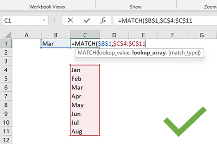
Arguments of MATCH function,

=MATCH(lookup_value,lookup_array,[match_type])

1. In match_type argument,

   1. Two options are there for exact match and approximate match.

   2. Default is approximate match, that means we can feed TRUE or 1.

   3. For exact match, we have to feed FALSE or 0.

   4. If we ignore that argument, approximate match will be done.

2. Lookup_array must be one-way array. For example, we can feed either 10 row * 1 column as lookup array or 1 row * 10 column as lookup array.

MATCH function gives the relative position of lookup_value in lookup_array.

In our case, lookup value is C2 cell, which is "Jan", this will be looked in the range B5:H5. match_type is zero, so it is the exact match. The MATCH function will deliver the relative position of "Jan", which is 2. This will be used as input for col_index_num in VLOOKUP function.

So, region central is found at the 5th row of our table and Jan month column is the 2nd column of the table and the intersection of 5th row and 2nd column is, value 247.

That's what extracted by VLOOKUP function and it is dynamic. If we change the region and month, formula will recalculate and deliver the correct result.

Method 2:

Two-way lookup using Index and Match.

Arguments of Index function,

=INDEX(array,row_num,[column_num])

The formula in D2 cell is,

=INDEX($C$6:$H$9,MATCH($B$2,$B$6:$B$9,0),MATCH($C$2,$C$5:$H$5,0))

In array argument, we fed the range C6:H9, which is slightly differs from the table_array argument in VLOOUP function, where we included the region column and fed the rangeB5:H9 as the table. This is because, the array argument in INDEX function expects, only the range, where the output resides. Then for the row and column, we can ask help from MATCH function.

Here, 1st MATCH is fed in the row_num argument, Which will take the B2 cell ("West") as the lookup value and then this value is looked up in the range B6:B9 by exact match option.

So, MATCH will deliver the relative position of "West" from the range B6:B9, which is 2.

This will be used as input for row_num argument.

2nd MATCH is fed in the col_num argument, which will take the C2 cell ("Mar") as the lookup value and then this will be looked up in the range C5:H5 by exact match option.

So, MATCH will deliver the relative position of "Mar" from the range C5:H5, which is 3.

This will be used as input for col_num argument.

Intersection of 2nd row and 3rd column in the range C6:H9 is E7, and so the INDEX function will deliver the range E7 and after evaluation it will throw the value 308.

Comparison between the 2 method:

VLOOUKUP function is considered to be the fastest when compared with INDEX function.

This is because in two-way lookup,

1. INDEX function uses 2 MATCH functions which will dent the speed of that function.

2. When we have larger data set of 1,50,000 rows or above, then INDEX function takes longer time for calculation, compared to VLOOKUP function.

3. Referring the whole column is not preferred by experts, but in the regular use if we refer the whole column in the array argument of INDEX function, it will take ages for calculation compared to VLOOKUP.

Capabilities of INDEX function is far better than VLOOKUP function.

1. Lookup value's column can be on any side of Matching value's column, and this is bit difficult in VLOOKUP function (There are some workarounds for this in VLOOKUP function, but this will slow down the process).

2. INDEX function will deliver the range as the output, and we can use this capability to create dynamic ranges using INDEX function, this is not possible in VLOOKUP function, because it delivers the value as the output.