

How to create Searchable Drop-down list in Excel - 2 Methods
- V E Meganathan
- May 9, 2024
- 4 min read
Today we are going to discuss about searchable drop-down list in excel. There are numerous methods to accomplish this task in excel. But here we are going to do this in 2 methods. When we have more than 30 cells in our validation range, it is tedious to look for our desired name in drop-down. At that time searchable drop-down list comes to rescue. Lot to learn, let's dive in.

We have customer names in the range F1:F37, Drop down provided in A1 cell.
Where, we can type short form of name and click on the drop-down button to fetch full names which contains A1 cell text. Then, we can select our desired name from list.
Let me start this from scratch,
Method 1 - Classic version:

In A1 cell type any short name, in our case I typed 'sm' and pressed enter.
Use below formula in E2 cell and drag the formula all the way down till E37 cell.
=IF(ISNUMBER(SEARCH($A$1,$F2)),MAX($E$1:E1)+1,0)
Let me de-construct this into smaller digestible pieces,
Core of this nested construction is SEARCH function,
Arguments of this function,
=SEARCH(find_text,within_text,[start_num])
This function finds the starting position of substring in main text. If it finds the substring, then it delivers number else throws an error.
Here, find_text is 'sm' and so we fed A1 cell,
within_text is the main text and so we fed F2 cell.
A1 cell content "sm", is found in F12 cell, so will evaluate the search function result in E12.


Cell value in F12 is 'Erin Smith' in which 'sm' resides at 6th position.
Wrap this inside ISNUMBER function, If the SEARCH function delivers number, then ISNUMBER delivers TRUE else it will deliver FALSE.
Wrap this Boolean value in IF function logical-test argument. Wherever we find the text, we add one to already existing maximum number else keep zero.
Earlier construction helped us to place the sequence number for matching names.
Now we are going to extract the matching names in B2 cell.
Use below formula in B2 cell,
=INDEX($F$2:$F$37,MATCH(ROWS($B$2:B2),$E$2:$E$37,0))
Arguments of INDEX function,
=INDEX(array,row_num,[column_num])
F2:F37 range fed in array argument,
For the row_num argument, we can get help from MATCH function,
=MATCH(lookup_value,lookup_array,[match_type])
in lookup_value argument ROWS($B$2:B2) is fed.
First reference of $B$2 cell is absolute reference,
2nd reference of B2 is not locked in both row and column and so it is relative reference.
Here 1 row is there in the range $B$2:B2 and so it will deliver 1.
If we drag the formula down, it will become ROWS($B$2:B3),
2 rows are there in the range $B$2:B3 and so it will deliver 2 and so on.
In lookup_array argument, $E$2:$E$37 is fed.
In B2 cell,

In lookup_array range, one is there in 11th position, and so match function will deliver 11.
In B3 cell,

In lookup_array range, two is there in 29th position, and so match function will deliver 29.
So, INDEX will pick 11th and 29th position from given array.

To accommodate all names, extend the formula in B2 cell till B37 cell.
Create Name for dynamic range:
In C2 cell use below formula,
=OFFSET($B$2,,,MAX($E$2:$E$37))
Arguments of OFFSET function,
=OFFSET(reference,rows,cols,[height],[width])
In reference argument, we fed B2 cell. This is the starting position of our resulting array.
Since we don't need to offset from our starting position, Ignore rows and cols argument.
In Height argument, we pick maximum value in E column. Ignore width argument, since we have only one column.

When we changed the A1 cell value, formula found 9 names which contains 'C'.
As of now, we travel in right direction.
we are going to add this formula in C2 cell into named range.
Copy the formula from C2 cell, then press shortcut key Ctrl + F3 to open 'Name Manager' dialog box. Click 'New' to open 'New Name' dialog box as shown below.

In Name section, we gave 'Search_Drop_Down' to name our dynamic range and paste the formula in 'Refers to' area and click OK.
Formula in C2 cell served its purpose, so we can delete that.
Drop-Down list in A1 cell:
Delete any contents in A1 cell and press short cut key Alt + D + L to open Data validation dialog box.

Click drop down in Allow section and select List option.
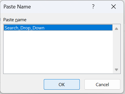
In source section. click inside and press shortcut key F3 to open paste name dialog box.
Select, recently created name 'Search_Drop_Down' and click OK.
Now in Data validation dialog box, select Error Alert tab and uncheck 'Show error alert' and click OK as shown below.

Change the font color in B2:B37 to white to hide from view.
Now in A1 cell type 'Ma' and select the drop-down, you can see that, it shows the names contains 'Ma' only. So, we don't have to look for all 36 names to pick one name.

Method 2 - Dynamic array:
In A1 cell type short name to be searched in our source data,
In our case type 'C' and use below formula in C2 cell,
=FILTER($F$2:$F$37,ISNUMBER(SEARCH($A$1,$F$2:$F$37)))

Argument of FILTER function,
=FILTER(array,include,[if_empty])
This function filters the range based on the criteria in include argument.
Output of include argument must be Boolean values or the resulting array can contain 1's and 0's. One is considered as TRUE and zero is FALSE.
Height of the range in array argument and include argument must be same.
If no matching records were found for given criteria, we can use third argument just like IFERROR function.
FILTER is dynamic spilled array function; you need to have 2019 or above version to access this. The formula will spill the result in adjacent cells. Formula resides in the first cell only.
If contents in other cells disturbs the spill range, then this function will throw an #Spill! error.
In SEARCH function within_text argument, we referred entire range with names instead of single cell. Then we wrapped the resulting array in ISNUMBER function as shown below.


These Boolean values will be used as filter criteria in array argument. Corresponding rows of TRUE will be considered in resulting array.
Use below formula in D2 cell,
=OFFSET($C$2,,,COUNTA($C$2:$C$37))
This is same as the earlier method, only difference is that we don't have the helper column to pick the maximum value in the height argument. So, we use COUNTA function to pick the count of matched names and fed it in height argument.
From now on this is same as earlier method, so we can follow steps from 'Create name for dynamic range' section in method 1.
留言