

How to extract text in Excel using text functions
- V E Meganathan
- Apr 24, 2024
- 3 min read
Today we are going to discuss about numerous methods in Excel to extract file name from file path using text functions. We will see text functions like MID, SUBSTITUTE, REPLACE, LEN, TRIM, FILTERXML. If we use ROW and INDIRECT construction with these text functions, then we can do unimaginable things in Excel. Lot to learn, let's dive in.

We will try to construct the robust solution, so that the same formula can be used to pick file names from different path. This is going to be an epic one.
Method 1:
Formula in C4 cell is,
=REPLACE($B4,1,SEARCH("@",SUBSTITUTE($B4,"\","@",LEN($B4)-LEN(SUBSTITUTE($B4,"\","")))),"")
Let me start this from scratch,
First, we are going to get the count of backslashes,
from that we are going to pick the last one,
then replace the backslash with some other text which we will not find in our file path for sure ("@"), and this is the starting point of file name.
Pick everything after "@" symbol.
How to get count of slashes in dynamic way?
Get overall length of text (consider that as L1)
Now, remove the slashes from text and get the length (consider that as L2).
The difference between the lengths L1 and L2 is the count of slashes. Simple mathematics.
The formula version of this,
=LEN($B4)-LEN(SUBSTITUTE($B4,"\",""))
Arguments of Substitute function are,
=SUBSTITUTE(text,old_text,new_text,[instance_num])
File path is fed in text argument,
"\" is the old text,
"" (Zero length text string) is fed in new_text argument,
instance number is optional argument, so we will ignore here.
Let me show you the result of this Substitute function,

Slashes are replaced with zero length text string, that means slashes are removed.
Length of this text is L2 and Length of B4 cell value is L1.
Count of slash = L1 - L2, is 6.
How to replace the Last slash with "@"?
SUBSTITUTE function is capable of replacing the text based on the instance number.
=SUBSTITUTE($B4,"\","@",LEN($B4)-LEN(SUBSTITUTE($B4,"\","")))

We simply used the count of slashes in instance_num argument.
In our resulting text, we have to find the position of "@".
=SEARCH("@",SUBSTITUTE($B4,"\","@",LEN($B4)-LEN(SUBSTITUTE($B4,"\",""))))

All we have to do is to remove the text from 1st string position, till the position of "@".
When we have start and end position to be replaced, then REPLACE function will help us,
Arguments of REPLACE function are,
=REPLACE(old_text,start_num,num_chars,new_text)
=REPLACE($B4,1,SEARCH("@",SUBSTITUTE($B4,"\","@",LEN($B4)-LEN(SUBSTITUTE($B4,"\","")))),"")
old text is B4 cell value,
Start_num is 1,
number of characters is the result of SEARCH function (Position of "@"),
New text is zero length text string ("").

Method 2:
In method 1, we removed text till "@" character.
But here, we are going to play with text after "@" character.
Formula in D4 cell is,
=MID($B4,SEARCH("@",SUBSTITUTE($B4,"\","@",LEN($B4)-LEN(SUBSTITUTE($B4,"\",""))))+1,50)
Let me de-construct this into digestible pieces.
Argument of MID function are,
=MID(text,start_num,num_chars)
This is same as method 1, till SEARCH function,

MID function helps us to extract the part of text.
start_num argument asks us where to start?
num_chars argument asks us how many characters to extract?
We know the starting position, but we are not sure about number of characters.
If we use larger number (maximum of 255), MID function is programmed to look for that much length and to give the available characters.
255 is kind of overkill for excel and so we decided to use 50 as number of characters.
In our case, we are sure that, we do not name the files more than 50 characters.

MID function includes the starting position character, so we add 1 in starting num argument,
Method 3:
Formula in E4 cell is,
=FILTERXML("<All><Text>"&SUBSTITUTE($B4,"\","</Text><Text>")&"</Text></All>","//Text[last()]")
Please visit below post to know more about FILTERXML function,
Method 4:
Formula in F4 cell is,
=TRIM(MID(SUBSTITUTE($B4,"\",REPT(" ",LEN($B4))),(LEN($B4)-LEN(SUBSTITUTE($B4,"\","")))*LEN($B4),LEN($B4)))
We already discussed about this method in below post,
Method 5:
Formula in G4 cell is,
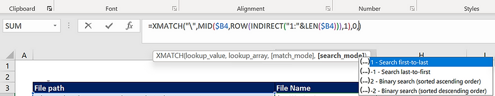
=MID($B4,XMATCH("\",MID(B4,ROW(INDIRECT("1:"&LEN($B4))),1),0,-1)+1,50)
You need excel version 2019 or above to have access for XMATCH function.
XMATCH in text parsing, that is great.
Let me de-construct this into smaller pieces,
Same old ROW/INDIRECT construction to get the sequence of numbers in dynamic way.
=ROW(INDIRECT("1:"&LEN($B4)))

=MID($B4,ROW(INDIRECT("1:"&LEN($B4))),1)
We use MID function to extract 1 character from 1st position, 2nd position and so on till
47th position.

Here, we have to find the position of last backslash. If we use MATCH function, it will find the position of first backslash and so we ask help from XMATCH function. It has the capability to search from last to first.
=XMATCH("\",MID($B4,ROW(INDIRECT("1:"&LEN($B4))),1),0,-1)
Argument of XMATCH function are,
=XMATCH(lookup_value,lookup_array,[match_mode],[search_mode])
in search mode argument, if we feed -1, it will do search from last to first,
Once we get the position of last backslash, this is same as method 2.

Comments