
In our previous post, we discussed about the same requirement with Index and Small function, but today we are going to discuss about INDEX and AGGREGATE function.
Lot to learn, let's dive into the topic.
Let me give you the glimpse of our requirement,

Range B4:F17 contains sample sales data with Product, Date, Unit Price, Quantity and Sales amount. In the cell K2, Products 'A','B','C','D' provided in Drop down.
Our requirement is to extract the records from B4:F17 matching with K2 cell.
We can get the multiple matches in different methods in excel, but here we are going to discuss INDEX and AGGREGATE function method.
Let's take a look at the formula in I5 cell,
=INDEX(B$5:B$17,AGGREGATE(15,6,((ROW($B$5:$B$17)-ROW($B$5)+1)/($B$5:$B$17=$K$2)),ROWS($I$5:I5)))

Let me deconstruct the AGGREGATE part, which is the core of this function.
Arguments of this function are,
=AGGREGATE(function_num,options,array,[k])
Argument - function_num:

This argument allows us to do 19 aggregate operations with list box facility to select desired operation as shown. Operations from 10 to 19 can handle arrays. If we drag the scroll bar down, we can see the options for large and small operations. The very same SMALL function which we discussed in our previous post, but here with much more ammunition. Option number for SMALL function is 15.
Argument - options:

This argument allows us to select 8 options.
In the next argument we will feed range or array, in that range or array, we have that option to ignore hidden rows, error values or subtotal function. Since, our construction in array argument will have error values for the records other than the matching records. we are going to use option 6.
Argument - array:
In the Array argument, we have two parts, numerator and denominator.
In the numerator part,
we can see that the same construction which we used in our last post to create the sequence of numbers.

Let me give you the glimpse of it again, The ROW function will deliver the Row number of given reference, If we feed B5 cell as the reference in ROW function, it will deliver 5. If we feed B5:B17 as the reference it will deliver the row numbers of that range, So the output will look like below.


If we detect the row of B5 which is 5, then the sequence will start from 0 and so we are adding 1 to it. This is the robust construction for sequence of numbers, so it will work even if we delete the rows.
In the denominator part,
we simply use the logical operation ($B$5:$B$17=$K$2)
What this operation does is that, it will check each cell in the range from B5 to B17, are you equal to K2 cell value. If yes, then it will deliver TRUE else FALSE.
After evaluation, the denominator looks like below,
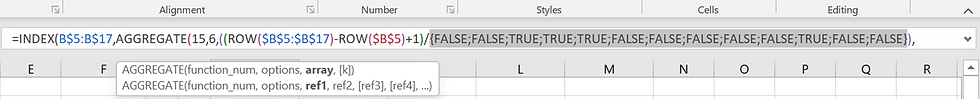
Now we are dividing the sequence of numbers from 1 to 13 by the sequence of TRUE's and FALSE. When we do mathematical operation on TRUE's and FALSE,
TRUE will be converted into 1 and FALSE will be converted into 0. Any number divided by one is same and any number divided by zero will throw divisional error. If we evaluate the array argument, it will look like below.

If we take a closer look at our data, we can see that 3, 4, 5 and 11 are the records match with K2 cell value which is 'B'.

Now everything falls in line, we did select option 6 to ignore error values. If we ignore errors in our resulting array, only the sequence of matching records are available which is 3, 4, 5 and 11. In the function_num argument, we picked option 15 which is SMALL function. It will give you the first small and 2nd small based on the [k] argument. To extract 1st small in that array, we can use ROWS function with expandable range,
First reference ($I$5) in rows function is locked in both row and column, it is absolute reference, It will not change as we drag the formula down or right. 2nd reference (I5) is not locked in both row and column, it is relative reference. In between the range I5:I5, how many rows are there ? only one and so the rows function will deliver 1, then small function will pick the first small of the array which is 3, If we drag the formula down, 2nd reference will change as I6, How many rows are there in the range $I$5:I6? 2 rows are there, and so rows function will deliver 2 and the small function will pick 2nd small in the array and so on.
Relative positions of product 'B' which is 3, 4, 5 and 11 are fed into the row_num argument of INDEX function and it will deliver the ranges corresponds to the relative postions from the range B5:B17, that means, B7, B8, B9 and B15.
If we drag the formula from I5 to J5, same relative postion of product 'B' will be used to extract Date.
Bonus Tip:
We dragged the formula for 4 rows to accommodate the records of product 'B', but product 'A' only contains 3 rows, so other row wil be full of errors as shown below.

To overcome this, we can add one condition in our already existing formula and one more additional formula as shown below. In E1 cell, get the count of each selected product using Countif function.


Comments