Method to repeat items based on count using excel formula

Today we are going to discuss about the method to repeat items based on count column using excel formula.

Let me show you the requirement and expected result.

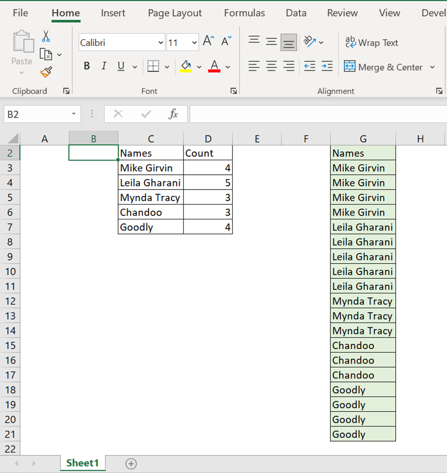
In the range C3:D7, names and count details are there in adjacent columns.

Our task is to repeat the names based on count. You can see that in the range G3:G21, 'Mike Girvin' is getting repeated 4 times and 'Leila Gharani' is getting repeated 5 times and so on.

Lot to learn, Lets dive in.

Formula in G3 cell is,

=INDEX($C$3:$C$7,MATCH(FALSE,COUNTIF($G$2:G2,$C$3:$C$7)=$D$3:$D$7,0))

If you are using excel version 2016 or earlier, Press Ctrl + Shift + Enter. Then you can see, the above formula is housed with curly braces like below.

{=INDEX($C$3:$C$7,MATCH(FALSE,COUNTIF($G$2:G2,$C$3:$C$7)=$D$3:$D$7,0))}

Let me deconstruct this into digestible blocks,

The core of this function lies at COUNTIF part, so let me start from there.

Arguments of COUNTIF function are,

=COUNTIF(range,criteria)

Will share one simple example to get an idea about this function,

This is exactly the opposite of our requirement; Names are there in the range B4:B22 with duplicates. We are going to get the number of occurrences of each name in E4:E8 range.

In COUINTIF function,

we feed B4:B22 in the range argument,

we feed D4 cell in criteria argument,

It will pick 'Mike Girvin' as the criteria and will count number of occurrences in B4:B22 range. 'Mike Girvin" is there for 4 times, and so on. If feed 2 criteria, then COUNTIF function will deliver 2 results for the count of each criterion as an array. This is the simplest form of Countif function.

Now we head back to our requirement.

In range argument, we feed $G$2:G2, this is the expandable range. First $G$2 reference is locked in both row and column, so it is absolute reference. This reference will not change as we drag the formula down. 2nd reference of G2 is not locked in both row and column, so it is relative reference. If we drag the formula one cell down, then it will become G3 and so on.

Here, $G$2:G2 is simply G2, and the value is 'Names'.

In criteria argument, we feed $C$3:$C$7, this is absolute reference. This reference will not change as we drag the formula down. Here, criteria count is 5 and so the result is 5*1 array.

COUNTIF function will pick each criteria and counts the occurrence in range.

First criteria is 'Mike Girvin' and the range value is 'Names',

Count of 'Mike Girvin' in 'Names' is zero and so COUNTIF function throws 0 and so on.

We do logical comparison 'equal to' operator ('=') with output of COUNTIF function and $D$3:$D$7 values. Result of this comparison will be Boolean value of TRUE and FALSE.

Each element in the first array is compared with each element in 2nd array.

Just to make you understand easily, the process of comparison shown below.

When we evaluate lookup_array argument of MATCH function by pressing F9 key, you can see that our simulation in left pic and evaluation in below pic provides same result.

In MATCH function,

Boolean value FALSE is used in lookup_value argument. When we match this lookup_value (FALSE) in list of FALSE in lookup_array, False is there in the first position in list and so MATCH will deliver 1 as output.

Then, INDEX function helps us to get 1st value from the range C3:C7, which is 'Mike Girvin'.

To get more clarity in the flow, we are going to evaluate part of formula in G7 cell. Because that's where name change occurs.

Take each criteria from the range C3:C7, and count the number of occurrences in the range.

'Mike Girvin' is there for 4 times; all the other names are there for 0 time.

We are going to compare this with count values in D3:D7.

Output of this comparison is shown below,

In the lookup_array, FALSE is in the 2nd position and so MATCH function will deliver 2,

INDEX function helps us to get the 2nd value from C3:C7 range, which is 'Leila Gharani'.

If we drag the formula all the way down, output will look like below.