Mysterious LOOKUP function in Excel from Basic to Advanced
- V E Meganathan
- Apr 29, 2024
- 3 min read
Today we are going to discuss about LOOKUP function in excel. This is all about LOOKUP from basic to advanced level. We will shed some light on this most underrated but yet powerful function. Lot to learn, let's dive in.
Example - 1:
Grade table is in the range F4:H9 - Lookup table.
Marks are in the range B4:B14,
We need to find the grade for each mark in the range C4:C14.
This is widely used form of LOOKUP function,
In lookup table, Min-Max is provided for understanding, we can keep that or remove that based on your requirement. Our lookup table is sorted based on maximum marks column in ascending order. This is the best scenario for approximate match lookup and so we ask help from LOOKUP function.
Arguments of LOOKUP function are,
=LOOKUP(lookup_value,lookup_vector,[result_vector])
=LOOKUP(lookup_value,array)
We can use this function in 2 ways, let me show you one example in each method.
LOOKUP with 3 arguments:
Formula in C4 cell is,
=LOOKUP(B4,$F$4:$F$9,$H$4:$H$9)
B4 cell value (75) is fed in lookup value argument,
Lookup vector is in the range F4:F9,
Result vector is in the range H4:H9.
In the lookup vector, this function will check the below condition in each row,
Is 0 greater than 75? No. then,
Is 16 greater than 75? No. then,
Is 26 greater then 75? No. then,
Is 41 greater then 75? No. then,
Is 61 greater then 75? No. then,
Is 81 greater then 75? Yes. then,
Go down and pick 61 which is in the 5th position in lookup vector.
So, this function will pick the value in 5th position in result vector which is "B".
That's how it does for each mark.
LOOKUP with 2 arguments:
Formula in C4 cell is,
=LOOKUP(B4,$F$4:$H$9)
Lookup value is B4 cell value,
Entire lookup table is fed in array argument,
First column in array is considered as lookup vector and last column in array considered as result vector. There is a criteria behind that, we will discuss at Example - 3. Then it works in the same way as above example.
Example - 2:
Text and numbers are there in one column, our task is to find the recent text or number.
This must be dynamic, if we add more text or number, then recent one need to be picked.
Last cell with text:
Formula in G4 cell is,
=LOOKUP("ZZZZZ",$D$5:$D$18)
Here, we used some larger text in terms of sorting, in lookup value argument.
Same concept of numbers comparison is applied here for text comparison.
Is 'Leila Gharani' greater than 'ZZZZZ' and so on. This comparison will go till D18. No text in this range is greater than 'ZZZZZ' and so this will come down and pick 'Jordan'.
As you can see in right side picture, this function picks new text value if we add data and this will ignore numbers.
Last cell with numbers:
Formula in G4 cell is,
=LOOKUP(99999,$D$5:$D$18)
Instead of text, we used some larger number in lookup value argument. Make sure that, no number in our data is greater than our lookup value.
This will ignore texts and will check only numbers, then it will pick the last value with numbers as shown below.
Example - 3:
LOOKUP function does VLOOKUP and HLOOKUP when it comes to approximate match lookup. But lookup table does the selection of VLOOKUP or HLOOKUP.
Here is the criterion:
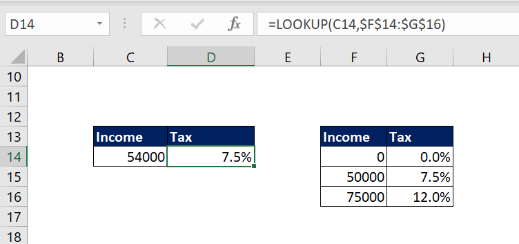
Let me explain with one example. Here, income tax rates given in the lookup table.
Our task is to find the income tax for given income.
Formula in D14 cell is,
=LOOKUP(C14,$C$6:$F$8)
Here, our lookup table size is 3 row * 4 Column.
So, number of rows is less than number of columns. In that case, LOOKUP function will do HLOOKUP and will give you the wrong result.
It will look for 54000 in 1st row, only 0's and texts are there in that row, so it will pick 0 in F6 cell as the lookup value and will deliver the F8 cell value as the output, that's why it delivers 12.0%.
Let me change the dimensions of lookup table to get the correct result.
Here, the lookup table size is 3 row * 2 column. If number of rows is greater than number of columns, then it is VLOOKUP.
So, we are getting correct result.


Comments