
Today we are going to discuss about pivot tables in excel. I will get you through in excel pivot tables from basic to advanced level. But for now, will share the basics.
Lot to learn, let's dive in.

This is the sample data; total data contains 9995 rows and 15 columns. Here, you can see first 20 rows of data to get some idea about source. You can use your own data; process will be same and so no need to worry.
Pivot tables helps us to summarize data in quick and easy way compared to other methods.
Just drag and drop the fields in Row, Column, Filter and Values area, then it will do summarization for you. Pivot tables are experts in giving the useful insights and patterns.
Basic rules for source data:
Column header or Field can't be blank.
Try to avoid duplicates in Field names.
No blank rows in between the data and No subtotals in between the data.
Select entire range or click in one cell anywhere in the range.
In menu bar, insert tab, Tables group, you can see PivotTable option click on that, 'Create PivotTable' dialog box will open. Else,

We can use Alt + N + V shortcut key to open 'Create PivotTable' dialog box.
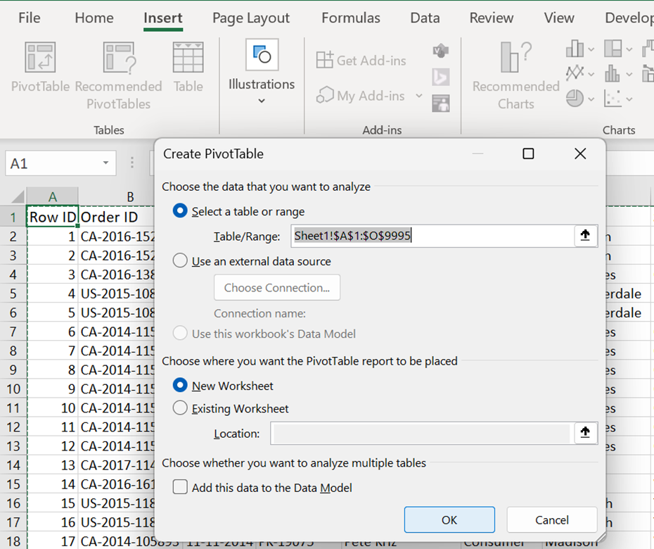
Check the table range in 'select a table or range' box, if the range is not picked properly, then you can change that by clicking on the up-arrow key. In 'Choose where you want the PivotTable report to be placed', select new sheet or existing sheet based on you preference. If it is new sheet, You can see that 'Location' option is disabled. It will place the Pivot table in default location in A3 cell. If we select 'Existing worksheet' then click on the
up-arrow key in location box and select your preferred sheet and location. In our case, I selected new worksheet.

In Sheet2 A3 cell, pivot table is inserted, in the right side, you can see 'pivot table fields' list and in the menu bar 2 tabs namely 'PivotTable Analyze', 'Design' got added, we call it contextual tabs. Pivot table fields list and contextual tabs are only visible if we click inside the pivot table. Even after clicking inside pivot table, if the pivot table field list is not visible, then click on the 'PivotTable Analyze' tab in menu, in right side, 'show' groups area, you can see 'Field List' option, click on that. It is a toggle key; it helps us to hide the fields list and to bring back the fields list.
Hover the mouse over the Pivot table fields as shown below, you can see that mouse cursor changed into 4 headed arrows, click there and drag the fields list wherever you want.


We can resize that based on our preferred size. In pivot table fields list, drop down is provided near gear icon, Click on that.
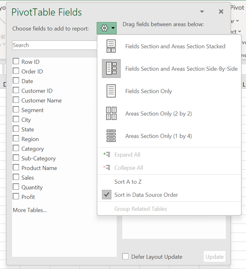
We can customize the design of fields list in different ways as shown in the picture.
By default, headers are sorted based on the source data order. When we have more headers in source data, we can use 'Sort A to Z' option at the bottom of the left picture to ease the field selection process.
Hover over the mouse again to top of the Pivot table fields, when we see the 4 headed arrow, click and drag all the way in right side and throw at the edge of the screen. Now you can see that, it got settled in its origin position.
Let me start the summarization,
We are going to raise questions to data and will try to find the solution using pivot tables.
Question 1:
Can you please show me the sales amount for each state?
Solution:
Here, we are going to calculate the sales amount and so the value field is 'Sales'.
Criteria which we are going to use is state and so the Row or Column field is 'State'.
Let me try the field 'State' in both row and column and will pick the suitable one.
To place the fields in any of the 4 sections, you can simply check the box on the column header, or you can simply drag and drop in the sections.


If we drag the 'State' Field into columns, then output is not readable, we have to scroll across 50 columns to see entire states. So, we can pick 'State' field in Rows as the best option.

Question 2:
Can you please show me Region wise profit with category split up?
Solution:
Insert New Pivot table in the 'Sheet2' in F3 cell.
Here, we are going to calculate the profit amount and so the value field is 'Profit'.
Criteria which we are going to use is region and category, so we can try Region in row, Category in column.

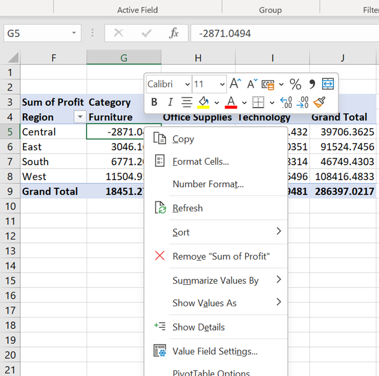
Number Formatting method:
Right click in any one of the cells with number and select 'Number Format' option.
Then, you can set the format based on your preference.
If we select, range of cells in pivot table and change the format using Ctrl + 1 shortcut key, then it will change the format only for that range, if region or category getting added in future months, no formatting will be there in those cells.

Question 3:
Can you please show me Monthly sales for each year?
Solution:
In our source data, we have 'Date' column, but here the requirement is to group the sales by month and year. We don't need to panic; we don't have to use any formulae. All we have to do is, drag and drop. If we drag the 'Date' field in row or column section, then pivot table will create the Hierarchy and will add the field for year, Month, Quarter. See the magic.

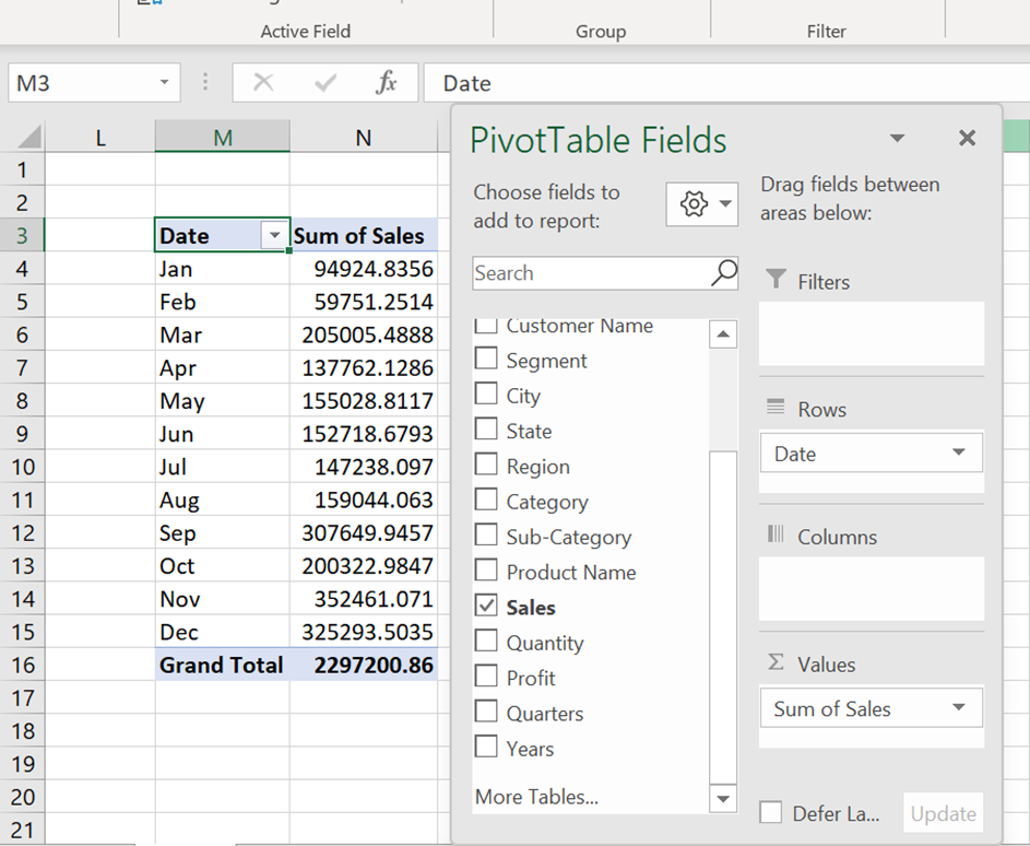
In the left side picture you can see the hierarchy in 'Rows' section. Now, we can simply remove years and Quarters from 'Rows' section. You can see that in right side picture.
Then, from the fields area drag the years into 'Columns' section and do the number formatting stuff.

Question 4:
can you please show me the average of sales in above pivot instead of sum of sales?
Solution:
This is not the formula solution to start from the scratch, this is Pivot table. All we have to do is 5 clicks.
There is a drop down in the values section after sum of sales, just click on that and select 'Value field settings' from the given options. Dialog box will open. in which select average in the list of 11 aggregate functions as shown below.
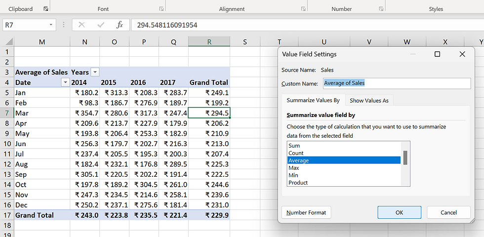
Now, what you see is the Average daily sales of each month for each year. Number format option is there in the left side of OK button, we can change the format here also.
This value field setting dialog box is like one stop shop, we can do all here.
At the center of dialog box, you can see ' Show values As' tab. There are lot of calculation options in that tab, we will see that in our next post.
Comments