

Unleashing the Power of Excel Function - SUMIFS: A Comprehensive Deep Dive
- V E Meganathan
- May 29, 2024
- 3 min read
Today we are going to discuss about SUMIFS function in Excel. In corporate world, Excel dashboards are flooded with 4 logical aggregation functions mainly are COUNTIF, SUMIF, COUNTIFS, SUMIFS.I will get you through from basic to advanced level in SUMIFS function.
Lot to learn, let's dive in.
SUMIFS function, sums the value column after applying filter criteria in multiple columns.
All filter criteria are applied in AND condition.
That means, each filter is applied in table to respective columns and sum operation will be carried out in value column only for those matching records.
Let me start with 2 criteria in 2 Columns:
Calculate the sum of Sales Amount for each Year and Quarter in below raw data.
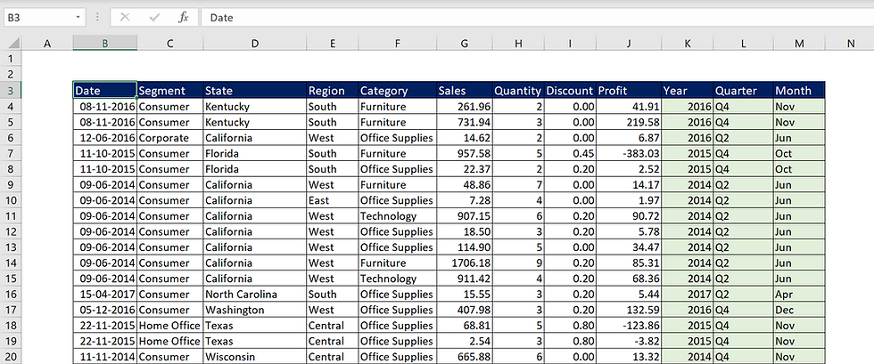
Sales amount is in G column,
Year, Quarter and Month are helper columns created with the help of date functions:
Year =YEAR(B4)
Quarter ="Q" &MONTH(MONTH(B4)*10)
Month =TEXT(B4,"mmm")
Arguments of SUMIFS function,
=SUMIFS(sum_range,criteria_range,criteria,...)
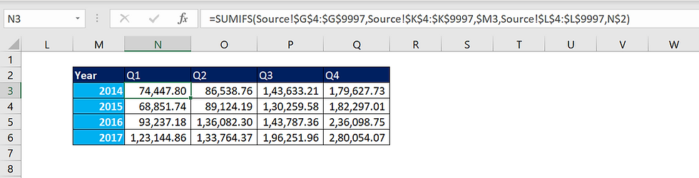
Formula in N3 cell is,
=SUMIFS(Source!$G$4:$G$9997,Source!$K$4:$K$9997,$M3,Source!$L$4:$L$9997,N$2)
Arguments are organized in the way that no explanation is required.
Sum range is G column,
Criteria range is K column which contains year,
So, criteria is M3 cell that is 2014.
Next criteria range is L column which contains Quarter,
So, criteria is N2 cell, that is Q1.
Let me compare the result by applying manual filters in source data for year 2014 and Quarter Q1.

Bonus Tips:
Size of sum range and criteria ranges must be same, otherwise this function will throw an error.
These ranges are compared with relative positions, so make sure the reference match and the size are same. For ex.,
Sum range contains G10:G25,
Criteria range contains G11:G26,
Since the size is same, function will start compare relatively and deliver incorrect result.
2 Criteria in same column with AND condition:
Calculate the sum of profit incurred between the dates 01/06/2016 and 31/10/2016.
Dates are in B column,
Profit data is in J column.
So, formula in O3 cell is,
=SUMIFS(Source!$J$4:$J$9997,Source!$B$4:$B$9997,$M3,Source!$B$4:$B$9997,$N3)

Here, criteria are placed in M3 and N3 cell with comparative operators in text format.
2 Criteria in same column with OR condition:
Calculate the Sum of Profit for the category Furniture or Technology.

In criteria argument, we fed both categories. But the function throws the sum of sales for each category not the sum of sales for both categories.
This is because, this function only accepts AND condition. More than one criterion in same column is an OR condition
No problem, we have some workarounds to overcome this. Just wrap this entire function in SUM function.

In that way, we forced SUMIFS function to accept OR condition.
Criteria with wild card character's:
Calculate sum of sales for any region which contains East in below raw data.

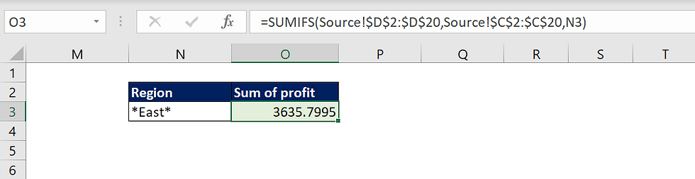
In N3 cell for criteria, '*' is used before and after 'East', that means, accept anything before and after 'East' as filter criteria.
'*' or asterisk is the wild card character which is used as the replacement for 'one or more characters'.
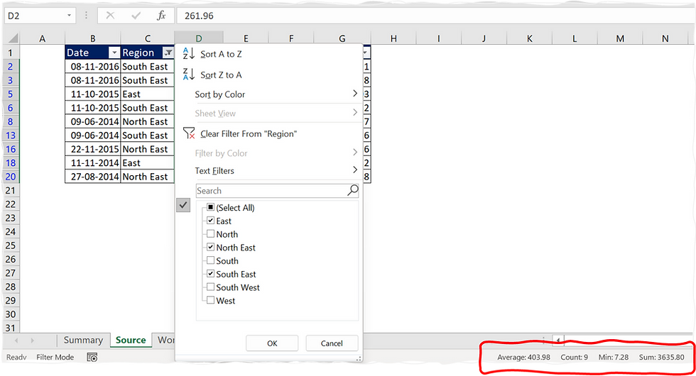
Let me check the result by applying manual filter.
What if we need to sum a range that spans multiple columns:
Calculate the sum of sales for all months where the sales are less than or equal to 100.
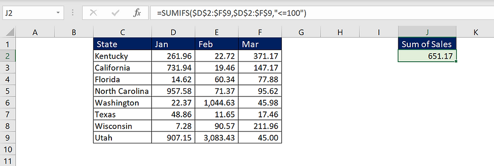
No issue, SUMIFS function can handle 2-dimensional range.
2-dimensional range as the result:
let me take our first requirement,
Calculate the sum of Sales Amount for each Year and Quarter in below raw data.

Single cell formula, which delivers 2-dimensional range as result. Formula resides in N3 cell, and it spills the results till Q6 cell.
Hozzászólások